When analyzing power in order to improve efficiency in electric devices and appliances, it can be beneficial to take a step back and look at the measurement instrument
Although efficiency has been replaced by effectiveness as favorite criterion in the business world, it still dominates the world of engineers and technicians. The hunt for improved utilization of electricity permeates every level in the electronics industry, from individual semiconductor components over circuits and modules to entire devices and even complex systems. While the exact definition of efficiency inevitably depends on the context, all variations have in common the consideration of results vs. effort, or in more technical terms, output vs. input.
Consequently, when aiming to improve efficiency, two possible approaches suggest themselves:
(I) Achieving the same output with less input (“doing the same with less”)
(II) Achieving more output with the same input (“doing more with the same”)
Of course, there are hybrid cases, e.g. when you have to increase the input by 10% to grow the output by 20%, but for simplicity’s sake we will subsume those scenarios under “doing more with the same”, since the bigger change occurs on the output side. In power electronics, the key variable is electrical efficiency, which defines the ratio of useful power output to total power input. Depending on the complexity of the device under test, there might be multiple stages of power conversion, which can all be evaluated separately. The principle remains the same, overall efficiency is a result of the concatenation of those partial efficiencies.
Extending the scope
Precisely measuring those efficiencies under all kinds of circumstances and operational conditions is a key purpose and raison d'être of dedicated power analyzers. Typically, when comparing analyzers, the accuracy of efficiency measurements – especially for taxing applications like variable frequency drives and the like – is the key metric for judging the instrument. This is necessary, but not sufficient. Why not extend efficiency considerations to the measurement process and the instrument itself?
The question “What do we get out of it for our investment?” is a reasonable one to ask, also regarding the power analyzer itself. In that scenario, the output consists of the results obtained by measuring, while the input is defined by the necessary investment to arrive at those results. The term ’investment’ is used in its broadest possible sense here, including time and effort as well as capital and operational expenses.
Power analyzers vastly differ in their number of channels, accuracy, bandwidth etc. For the purpose at hand, let us assume those models not capable of producing the target output with sufficient accuracy have already been weeded out. Thus, we can focus on the input side of measurement efficiency: the total investment required to generate the output.
Since power analyzers with similar specifications are generally in a similar price range, let us also exclude hardware costs from our considerations from here on. The bulk of the remaining investment is made up by the engineers’ time to carry out the required measurements. Generally, once the setup is completed, the largest influence on total measuring time is the number of measurements. Twice the number of unique operating points to characterize, twice the time.
There are certain scenarios, however, that demand at least twice the effort per point than others. Sometimes, it is required to repeat the measurement with exactly the same settings of the DUT. When does this occur, and is there a way to avoid it?
Analyzing variable frequency drives
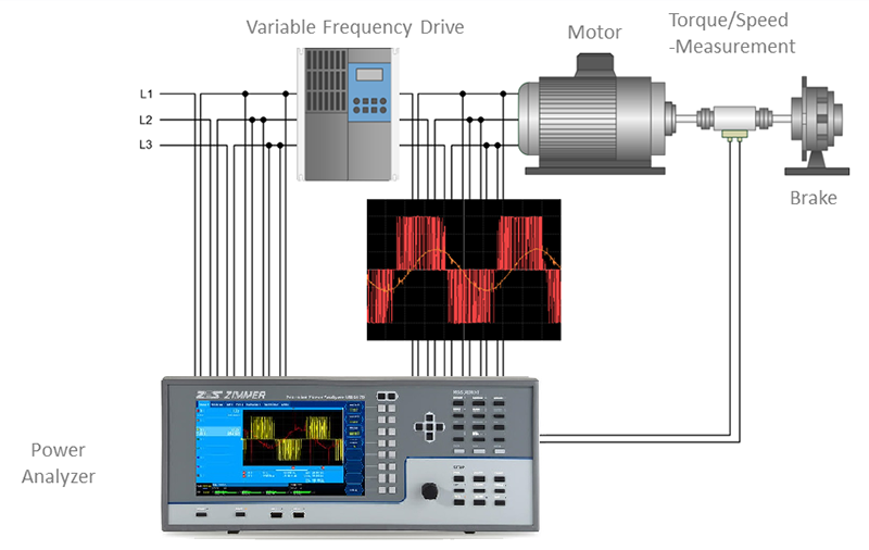
A prime example is the analysis of electric drive systems, as depicted in the exemplary setup of Figure 1. In order to measure the total power output e.g. of a variable frequency drive (VFD), the measurement bandwidth should be as broad as possible in order to capture high-frequency byproducts of the switching frequency.
Click image to enlarge
Fig. 1: VFD power measurement setup
Figure 2 shows an example power spectrum of a frequency converter with harmonics of the switching frequency and other side effects on the right hand side. For those type of measurements, all available filters should be deactivated to avoid unnecessary truncation of the spectrum. Even the anti-aliasing filters (AAF)? Yes, since there is no danger of aliasing when determining power – this is an issue frequently misunderstood.

Click image to enlarge
Fig. 2: VFD power spectrum
People often cite the Nyquist–Shannon sampling theorem, arguing that e.g. an analog bandwidth of 5 MHz is pointless with a sampling rate of 1MS/s, since all frequencies above 500 kHz are no longer accurately represented by the sample values. This is only half true: according to the theorem, you can no longer accurately reconstruct the original wave shape, if the sampling rate falls below half the signal frequency. The good news is: for power measurements you do not have to.
Power measurement with a digital power analyzer is a statistical process which can roughly be described as averaging over a large enough number of samples. You need to make sure you actually hit the wave at a sufficient number of points when sampling, and you also need to be careful not to always hit it at the same phase angle. The latter can be avoided by intelligent choice of the sampling rate in relation to the frequency of the signal. This is sufficient for correct power measurement, there is no need to reconstruct the exact shape of the signal. After all, there is an infinite number of different signals that all end up having the same power value.
Same DUT, different setup
Power is not the only relevant result when characterizing VFDs. For deeper analysis of the DUT’s behavior, e.g. with respect to causes of power leakage and electromagnetic compatibility, harmonic analysis is inevitable. And all of a sudden the Nyquist–Shannon theorem becomes relevant. Statistical averaging is no longer good enough when it comes to judging the frequency distribution of the signal.
We can turn the above argument upside down and state that many signals with exactly the same power can have wildly differing spectra. In order to precisely measure the harmonic content of a given signal, we have to be very careful to eliminate any content with a frequency above half the sampling rate. Otherwise, that portion of the signal would be undersampled and erroneously reconstructed as lower-frequency content, thus distorting the true power spectrum.
Let us consider a VFD with a switching frequency of 40 kHz as an example, using a power analyzer with a 1 MS/s sample rate. By proper use of an AAF, any signal content above 500 kHz will be removed, and the remainder will be analyzed properly in accordance with the sampling theorem. Harmonic analysis is possible up to the 12th harmonic at 480 kHz. The results of the analysis will be free from aliasing.
Deactivating the AAF will create an entirely different picture: all frequencies above 500 kHz will be misrepresented. The 13th harmonic will appear at 480 kHz after sampling and thus erroneously added to the 12th. The 14th harmonic at 560 kHz will be interpreted as 440 kHz and thus added to the 11th harmonic, the 14th will be added to the 10th etc. In short: the results will be completely invalid. After sampling, there is no way to distinguish the true harmonics from the mirror images created by aliasing. Filtering at this point is useless, at least for the purpose of the prevention of aliasing.
Testing time vs. hardware cost
The above illustrates that if we want to obtain both power and harmonics results, we have to employ two mutually excluding instrument setups, one with and one without AAF. The most common approach is to start without filters for power measurement, and then to repeat the procedure with filters for harmonic analysis.
“Repetition” has to be taken with a grain of salt, though, since it is as good as impossible to reproduce the exact same point of operation twice . An alternative is to measure the same signal on two power analyzers with different filter settings in parallel, but the cost for doubled measurement hardware renders this solution rather unattractive. Therefore, serial repetition is the most widespread approach.
While investing twice the time seems less painful than spending twice the money, it is still fairly inefficient, since there is a huge overlap between the two series of measurements – the only difference being initial activation or deactivation of the AAF. As the main purpose of using power analyzers is to reach new pinnacles of efficiency for the device under test, it is quite unsatisfactory to use a measurement procedure that is rather inefficient in itself. Therefore, we have often been challenged by our customers, most of whom share a predilection for efficiency, to find a way out of this dilemma.
It should be noted that it is not completely unheard of that the danger of aliasing gets consciously ignored, although such approach completely voids the purpose of precision power measurement in the first place. There is no point in choosing a sophisticated instrument while arbitrarily introducing an error of unknown magnitude to the measurements.
Engineering the solution
When designing our latest generation of power, it was clear to us that doubling all hardware components was out of the question, and it was also clear that the Nyquist–Shannon theorem presented a barrier not easily overcome. A closer look at the situation revealed, however, that the only functional part of the instrument required twice for taking both desired measurements at the same time was the sampling stage. All subsequent processing could be left mostly unaltered.
Instead of measuring with two instruments, it is sufficient to split the incoming signal, feed it into two independent analog-to-digital converters, and process the output accordingly. One of the signals thus obtained needs to be bandwidth limited before sampling in order to avoid aliasing, as described above in the section explaining the requirements of harmonic analysis.
We have named this novel architecture DualPath to highlight the hardware implementation of two completely independent signal paths already prior to sampling (See figure 3). The placement of the AAF before the analog-to-digital converter cannot be emphasized enough, as the order cannot be reversed: it is not allowed to sample first and filter later, thus splitting the signal stream only after sampling. While this approach obviously would turn out cheaper in terms of hardware costs, it violates the Nyquist–Shannon theorem and produces the kind of measurement errors described in the paragraph about harmonic analysis.

Click image to enlarge
Fig. 3. DualPath implementation ot two completely independent signal paths
A considerable impact
Returning to the initial reflections on efficiency in test and measurement, it is clear that a 50% reduction in measuring time has a considerable impact on the overall effort to obtain efficiency values for the DUT. While the time required for setup and configuration cannot be neglected entirely, it typically exerts a lesser influence.
Since efficiency measurements form part of a feedback loop implemented to optimize the design of the DUT, any reduction in test time directly results in more time to be spent on the actual design. Thus, improving the measurement efficiency of the power analyzer, as defined above, through better parallelization of measurements contributes to improved efficiency of the DUT itself.