Some history and loose ends
Current-mode control has been around in one form or another for almost 50 years now, but it is still a topic that creates much confusion in the minds of many engineers and researchers. In this series of articles, Dr. Ridley shows historical reasons for the confusion, and presents for the first time the source of past discrepancies in various research papers.
Current-mode control circuit
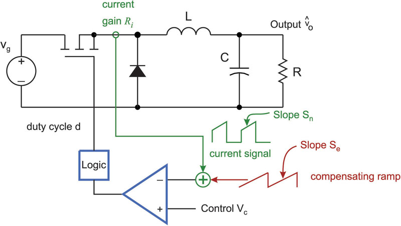
Figure 1 shows a buck converter with peak current-mode control. The instantaneous value of the current is added to a compensating ramp, and compared to a control reference, v_c. This implementation of current-mode control provides the most bandwidth and best performance, but results in the well-known problem of subharmonic oscillation.
The wide bandwidth of current-mode, and the oscillation problem, present problems in using a simple model for analyzing the system. This resulted in a considerable array of different analysis approaches which caused a great deal of confusion to both industry and academics.
Click image to enlarge
Figure 1: Buck Converter with Current-Mode Control
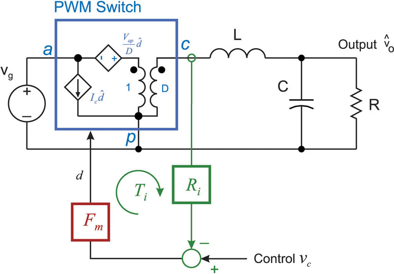
The early approaches to current-mode analysis took the same approach as for a voltage-mode converter. In the early days, this meant state-space averaging. Later on, the PWM switch model provided a simpler approach. Figure 2 shows the average model for a buck converter with current-mode control. A feedback loop around the inductor current represents the system. R_i is the gain from inductor current (or switch current) to the voltage signal input to the comparator. This may be just a simple resistor, or a current transformer with a resistor.
Click image to enlarge
Figure 2: Average Model of the Current-Mode Buck Converter
Early discrepancies arose in determining the gain of the current-mode modulator, F_m. Confusion continues to this day with research and industry papers, and it is very important to resolve these differences, and to find out why researchers found different values. This was discussed in [1], but the source of the discrepancies has never been published.
Figure 3 summarizes the most common approaches being used in the industry in 1986. There were no less than SIX completely different approaches results presented at this time, all of them from respected sources.

Click image to enlarge
Figure 3: Different Analysis Approaches Prevalent in 1986
Infinite-Gain Models
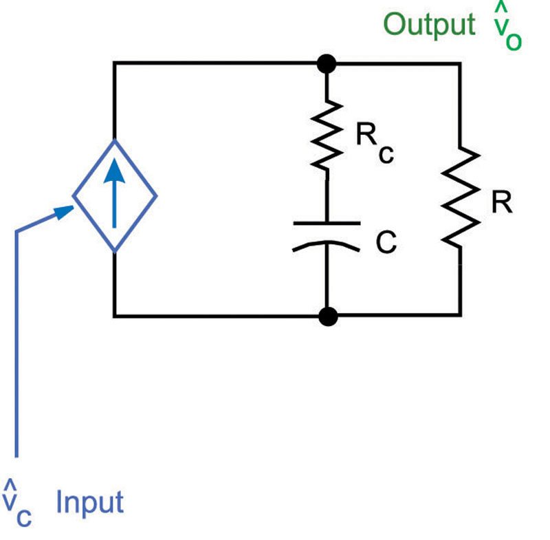
Probably the most universal approach used by industry appeared in the Unitrode Handbook and application notes. If the gain around the inductor current is assumed to be infinite, we can treat the inductor as a current source. This follows the logic of the current following the reference by the action of the comparator.
Figure 4 shows the resulting model. The controlled current source feeds the RC load, and the resulting model is first order.
Click image to enlarge
Figure 4: Current-Source Model Feeding Load and Capacitor
There is a problem to this approach, however. It is well known that current-mode control exhibits a subharmonic oscillation problem as the duty cycle approaches 50%. The waveforms exhibiting this problem are shown in Figure 5. The top set of inductor-current waveforms show growing oscillations at greater than 50% duty cycle. The lower set shows decaying oscillations when the duty cycle is less than 50%.

Click image to enlarge
Figure 5: Subharmonic Oscillation of Current-Mode Control
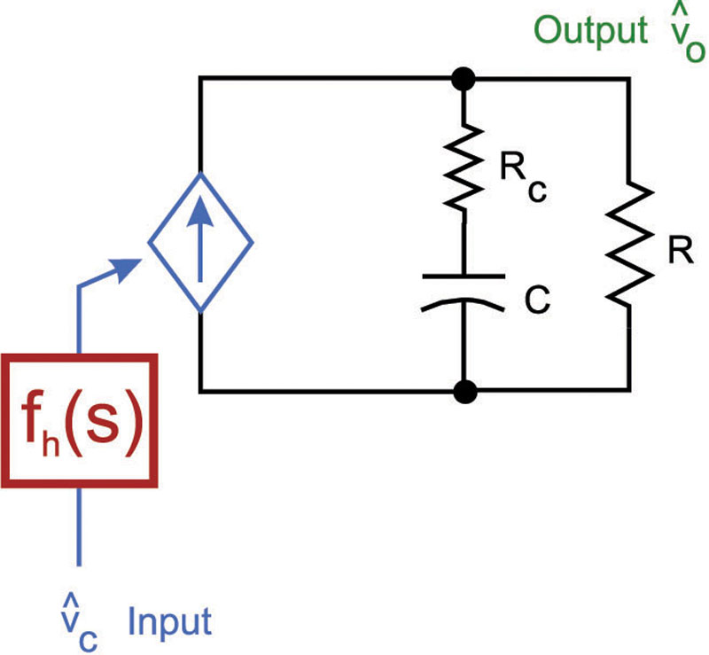
An engineer at Unitrode, Barney Holland, recognized this long ago in a paper, and proposed a refinement to the current-source model. He suggested that the oscillation exhibited the same characteristic as an LC filter tuned to half the switching frequency. A pair of double poles for the block f_h (s) can be used to model this behavior. Holland was quite correct in his observation, but it seems that his concept of using a three-pole representation for an LC circuit was not something Unitrode wanted to embrace, and no analysis followed on with this idea.
Even when the extra transfer function block is included in Figure 4, the gain of the current loop is assume to be infinite, and the current-source part of the model is preserved.
Click image to enlarge
Figure 6: Current-Source Model Feeding Load and Capacitor with Added Double Poles
Finite-Gain Models
Other researchers around the world recognized that the gain around the current loop could not be infinite, since the current in the inductor did not perfectly track the reference. The peak value of the current was an exact match, but the average current was not. Different way of analyzing the peak-to-average current then resulted in at least three different solutions for the finite modulator gain, F_m. Vince Bello, an independent engineer who produced many popular early Spice models, found one value of gain. Dr. David Middlebrook of Caltech found a gain which was twice as large (in the absence of a compensating ramp). Dr. Fred Lee, of Virginia Tech, found another much-larger value which could even approach infinity as the duty cycle approached 50%.
This was a very unusual situation. A single apparently-simple circuit produced some widely different analysis results. The dissertation of [1] addressed this issue, but it did not attempt to find out where the variations and discrepancies came from. As a result, to this day papers continue to be produced which use one of the four options for modulator gain, and there is no consensus of agreement.
A final analysis approach is shown in Figure 3. The precise discrete-time approach used by Dr. Art Brown produces very accurate results, but was too complex to be accepted by either researchers or industry. This model also used one of the same gains of the average models.
Summary
Multiple analyses of current-mode control continue to be derived, using one of four possible values for the gain of the modulator. In this article, we have shown the models resulting from an assumption of infinite current-loop gain. In the continuation of this series, we will look at other values which can result, and show how different analysis approaches can provide different results without any apparent errors. Finally, it will be shown how a shift in the analysis point can make all of the derivations converge to a single result.
References
[1] “A New Small-Signal Model for Current-Mode Control”. Full original version available as a free download at www.ridleyengineering.com/books.html. Updated color version available from Researchgate.
www.researchgate.net/publication/280491161_Current-Mode_Chapter_1 www.researchgate.net/publication/280491229_Current_Mode_Chapter_2
www.researchgate.net/publication/280682067_Current-Mode_Chapter_3
[2] Power supply design articles www.ridleyengineering.com/design-center.html
[3] Join our LinkedIn group titled “Power Supply Design Center”. Noncommercial site with over 5850 helpful members with lots of theoretical and practical experience. www.linkedin.com/groups?&gid=4860717
[4]See our videos on power supply design at www.youtube.com/channel/UC4fShOOg9sg_SIaLAeVq19Q
[5]Learn about current-mode control in our Power Supply Design Workshops www.ridleyengineering.com/workshops.html
 Single.jpeg)