Choosing the right power supply
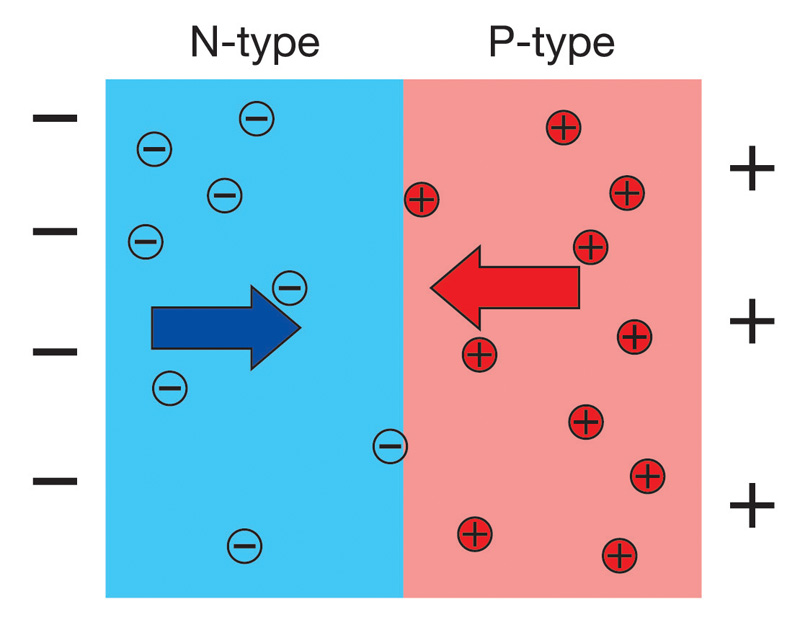
Figure 1: N and P type doping of an LED
LEDs are fast replacing Fluorescent light bulbs and incandescent light bulbs in many lighting applications. In the past these sources could be driven directly from the mains voltage, but this is not possible with LEDs. This paper looks at what an LED is, how to drive it, and also how to choose the right power supply for this requirement. Like any regular diodes, LEDs are constructed using a semiconducting material which has been �doped' with impurities in order to create a p-n (positive-negative) junction. Current flows easily from the p-side (anode) to the n-side (cathode), but not in the other direction. When placed in a circuit supplied by an external power source, current flows, and charge carriers (electrons and holes) flow into this junction from the electrodes which are at different voltages. The electrons and holes are separated by an energy difference known as a �band gap'. When an electron meets a hole, it falls across the band gap from the higher to the lower energy level, releasing the band gap energy as a photon of light with a frequency, and hence a colour that corresponds to the band gap energy. This relationship can be expressed using the following equation: Eg = hc/? Where: Eg = Band gap energy h = Planck's constant c = Speed of Light
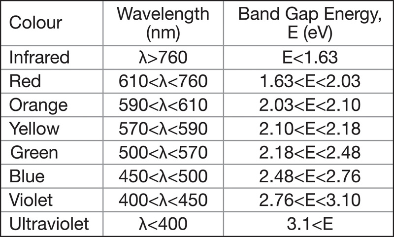
Table 1 shows the wavelengths and band gap energies of a number of coloured lights. LED manufacturers can �tune' the band gap energy and hence the wavelength of the light emitted. This is achieved by increasing or decreasing the level of impurities, controlling the composition of the semiconductor. Adding more impurities will lower the band gap energy, and so will increase the wavelength of the emitted light. The band gap of an LED changes with varying temperature, and the extent of this change can be predicted using Varshni's parameters (empirically measured values which are used in order to calculate temperature dependant band gap energies). This relationship is described in the following equation: Eg = Eg|T=0 K - ?T2/T+? where Eg = Band gap energy T = Temperature (K) ?, ? = Varshni parameters Since both ? and ? are constants for a specified LED, as temperature increases, the band gap energy of the LED slightly decreases. As seen previously, decreasing the band gap energy will increase the wavelength of emitted light, will slightly change the colour of the light emitted. This is referred to as temperature dependant spectral shift. Performance Characteristics of LEDs The voltage - current relationship of LEDs is given by Shockley's diode equation: I = Is(exp(VD/nVT)-1) VT = kT/q where I = Diode forward current Is = Reverse bias saturation current VD = Diode forward voltage n = Diode ideality factor VT = Thermal voltage k = Boltzman's constant q = Charge on an electron T = Temperature Since n, k, q and Is are constant for a given LED at a fixed temperature T, the V-I curve of an LED can be plotted using this equation as in Figure 2:
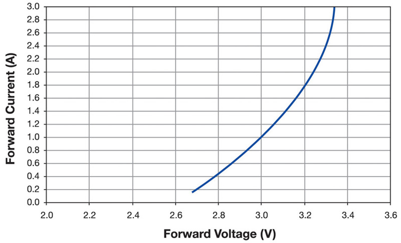
Shockley's equation also tells us that the forward voltage of the LED is temperature dependant. For a fixed forward current, as the temperature increases, the forward voltage of the LED decreases. This is because the saturation current Is is also dependant on temperature and can be estimated using the following equation: Is(T2) = Is(T1)exp[ks(T2-T1)]
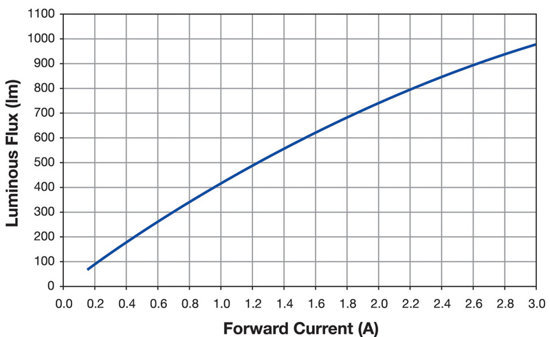
Next if we look at the empirical data of the characteristic luminous flux - current curve (Figure 3), and luminous flux - temperature curve (Figure 4) of an LED, we can draw two important conclusions:
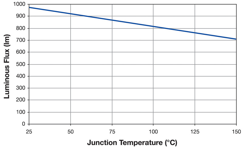
1. LEDs operate much more efficiently (they possess a much higher lum/W value) at lower current levels. As an example, we can use the figures for Cree's XM-L high flux LEDs. When driving the LED at 3 A (and at 25°C), it will emit 976 lumens. The power required to do so is 3 A * 3.34 V, or 10.02 W, resulting in an efficiency of 97.4 lm/W. However, when the LED is driven at 1.5 A, it will emit 590 lumens. The power required to do so is 1.5A * 3.14V, or 4.71W, resulting in an efficiency of 125.3 lm/W, a significant improvement. This higher efficiency means that there is less waste heat generated by the LED (self-heating) at lower currents which can alter both the wavelength and intensity of the emitted light as well as altering the forward voltage by raising the junction temperature. 2. An increase in temperature will decrease the forward voltage (and power) needed to maintain a constant current. However the lumen output will also fall, and by a greater scale. This means that that even though less power is required to maintain a constant current level; the lower lumen output will mean that the overall efficiency of the LED will fall. Why use a driver for LEDs Choosing the right supply is key to ensuring that you get the best performance from your LED. LEDs with their long lifetimes now mean that the perception is that the weakest link is now the power supply. Excelsys has chosen design techniques, market leading components and thermal management techniques in order to provide solutions for customers with lifetime matching figures. We also have incorporated a number of design features which fit in nicely with the LED market requirements. Constant current or constant voltage driver We have already stated above that LEDs are current driven devices, so why do companies offer both Constant Current (CC) and Constant Voltage (CV) solutions for LED drivers. The reason for this is to give the light fixture designers a number of options in optimizing their system. If many strings of LEDs are used in series, then the most efficient way to drive them is to use a constant current power supply, and connect the LEDs directly across the terminals of the power supply. However if strings of LEDs are connected in parallel then you may have an issue in trying to match the current in all the strings. A possible alternative to this would be to place an external component or active device to control the current. This may result in a slightly less efficient overall number of luminaires per Watt, but it allows the user to have full flexibility in ensuring that an identical current flows though many LED strings in parallel.
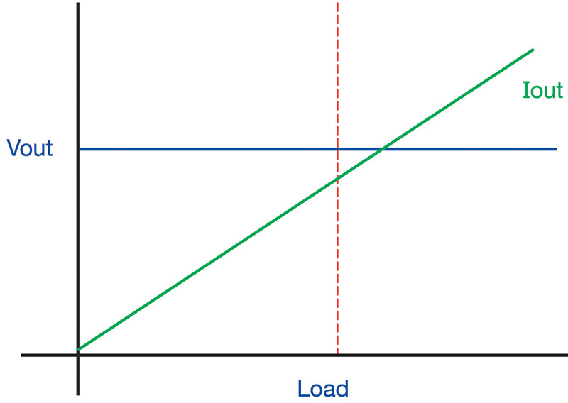
CC mode and CV mode Figure 5 to 7 show the characteristic of three distinct mode of operation of a power supply. On each plot the axis are the same. The X axis shows the load increasing, and the Y axis shows the output voltage of the module. The blue line is the voltage and the green line is the output current. You will note the performance of Constant Voltage power supply in figure 5. It shows as the terminology suggests a unit that delivers a constant voltage as the load increases. The load current rises as demanded by the system, and will continue to increase to a point where the power supply will go into current limit mode in order to prevent damage to the power train. In our catalogue this is represented by the LDV and LXV product ranges. A lot of common voltage requirements are covered by these ranges such , and some not so common voltages.
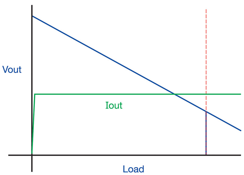
Fig 6 shows how a constant current driver will behave. As the load increases the output current will remain fixed, with the voltage decreasing accordingly. This is covered by our LDC , LXC and LXD product ranges.
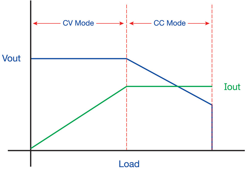
The latest design from Excelsys takes the two mode of operation and combines them onto one design. From figure 7 you can see how the unit will initially behave as a constant voltage unit. Once the load current max is reached, the control loop will then hold the supply current at a constant value and reduce the output voltage accordingly. This type of approach has many benefits to the end designer in that if chosen correctly both CC and CV mode designs can be achievable with one supply. www.excelsys.com
 Single.jpeg)