Predicting magnetics-winding proximity losses

In this special article we’ll look on work resulting from Ridley Engineering’s magnetics presentations at APEC 2016. Among things shown is how a linear circuit model can be used inside any version of Spice (or other circuit simulator) to get accurate results for the ac proximity loss resistance of magnetics windings. The equivalent circuit is derived directly from the physical structure of the windings and supported by measurements. This important work makes the findings of Dowell’s equations easily accessible to any engineer.

Inductor circuit model

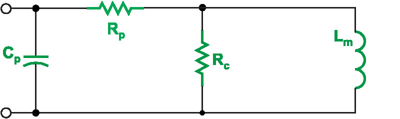
Figure 1 shows the traditional, and quite simple, circuit model for a high-frequency inductor. This equivalent circuit has been used for over 100 years to characterize the important constituent components of an inductor.

Click image to enlarge

Figure 1: Traditional Inductor Equivalent Model

For quite some time, power supply engineers have been using simple circuit models like these to simulate their power converter circuits. Unfortunately, the simulations fall short of observed reality, especially in the area of power dissipation. Simulated inductors simply do not have the same temperature rise as the real inductors in the circuit. This can lead to unexpected failures or greatly-shortened product lifetimes.

This problem has become more exaggerated in the last decade as many off-the-shelf inductors are now available, and designers push to higher frequencies with high ripple currents in the inductors. This is being done in an effort to minimize the inductor size. Not paying attention to ac resistance can be a fatal error.

More complete inductor circuit model

We have told design engineers many times that a much more complex circuit model is needed if you want to be able to get better simulation results for inductors. Generally, we have thought that the magnetics models are simply too complex for a circuit simulator to be able to handle them effectively.

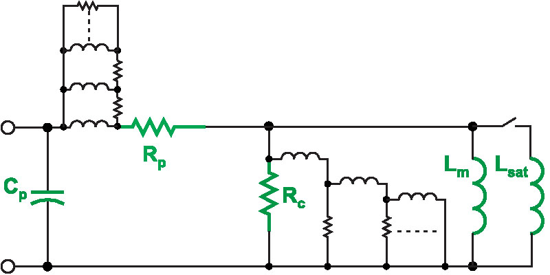
At the recent APEC conference in Long Beach, California, we presented what I thought was the minimum-complexity model needed to approach reality in simulation. This circuit is shown in Figure 2, although even this circuit is a little simplified for clarity in this article.

Click image to enlarge

Figure 2: More Complex Model Needed to Capture Most of the Important Behavior of Inductors

There are several modifications in this circuit compared to the standard circuit model used in the past. Firstly, the fixed inductor value is replaced with two discrete and different values – if the current through the main inductance exceeds the saturation level, a second and much lower value is used to represent how much inductance is left after the core is saturated. In reality, there would need to be a continuously-variable value of inductance with current, but two discrete values can often be sufficient to model many of the important phenomena that can occur with inductor saturation.

Secondly the core loss resistor, usually just a fixed value, is replaced with a ladder R-L network to represent the frequency-dependent nature of the core loss. The resistances of this network would also need to be modulated with the amplitude of the drive to the core, but that is beyond the scope of this article. Details of the derivation of the frequency dependent core loss model are given in [1].

Very few people usie such a model to simulate core loss properly – most usually just calculate the core loss separately from the circuit waveforms and the flux swing in the core on each cycle. This can provide reasonable accurate figures for the core dissipation although the calculations are usually time-consuming.

The third major modification to the traditional inductor circuit is the inclusion of a network to represent the frequency-dependent nature of the winding resistance referred to as proximity loss. This is shown as another ladder network to the left of the circuit.

Inductor model with proximity circuit added

For the rest of this article, we are going to focus on the winding losses of the inductor. It was discovered long ago that the resistance of inductor windings at high frequencies can be much higher than the dc resistance values.

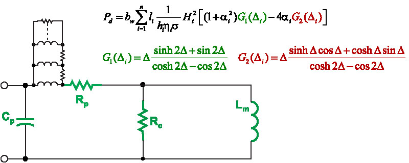
In 1966, Dowell published his famous equations for calculating proximity losses, and these are shown in part in Figure 3. Dowell’s equations show how the ac resistance can be tens or even hundreds of times higher than expected, and this is a not-subtle effect [2]. Despite the profound impact of the analysis, probably less than 1% of power designers ever use Dowell’s equations – they are simply too complex for most to understand and use in their day-to-day design lives.

Click image to enlarge

Figure 3: Traditional Inductor Model with Proximity Loss Circuit and Proximity Equations

When we presented the complex magnetics model of Figure 2 at APEC, I expected people to nod their heads and say, yes, that is too complex a model to even begin to expect Spice to be able to handle efficiently. Instead there was a very different reaction. Everyone wanted to know if the proximity loss circuit model could be generated automatically from either the physical structure of the windings, or from a measurement itself. If it could, then everyone could benefit from Dowell’s equations without having to fully comprehend and implement them directly. It turns out that this is completely possible, and that is not that difficult a task.

Predicted and measured AC resistance

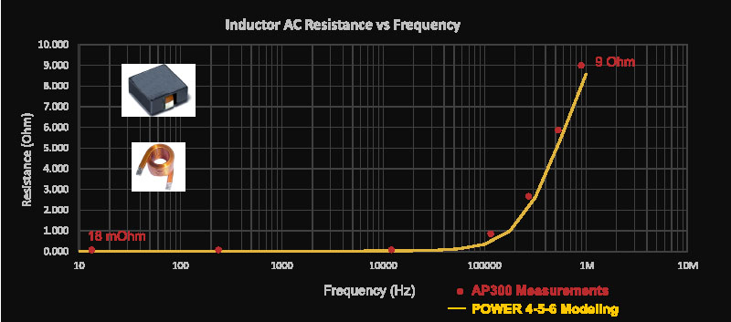
Figure 4 shows an off-the-shelf inductor with helical windings. This kind of inductor works well for applications where there is a a strong ac components, and also significant ripple current.  For this structure, the program POWER 4-5-6 [3] finds the solution to Dowell’s equation at multiple frequencies from dc to 100 times the switching frequency. The resulting ac resistance is plotted in the graph of Figure 4.

Click image to enlarge

Figure 4: Predicted and Measured AC Resistance of Helical-Wound Inductor

You can see the dramatic effect of the proximity analysis. The dc resistance is just 18 mOhm, but at 1 MHz the winding resistance has risen to 9 ohms, a 450 times increase! This does not necessarily mean that the inductor is not a good one – its main function is to carry dc current, and the harmonic currents must be considered individually to see how severe the heating problem will be.

It is essential to consider Dowell’s equation in your design. Figure 4 also shows measurements of the ac resistance of the inductor, made with an AP300 frequency response analyzer. The correlation between measurement and theory are very close for this inductor.

Linear circuit model

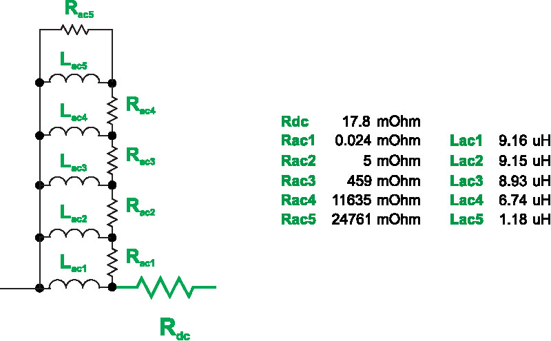
Figure 5 shows a linear circuit model that can be used to synthesize the changing values of ac resistance with frequency. A 5-step ladder network was chosen to model the ac resistance accurately to 10 MHz, well beyond the range of the inductor current harmonics. The circuit values are also given.

Clcik image to enlarge

Figure 5: Final Linear Circuit Model For Predicting AC Proximity Losses

At low frequencies the inductor impedances of the model are zero, so all the current flows through the dc resistance. As the frequency goes up, the current is steered through increasingly higher resistive branches, effectively raising the ac resistance.

This final linear circuit can be run in several ways. If it is driven with an ac source you can generate the ac impedance of the network which confirms the measured and predicted ac resistance. Secondly, an inductor current transient waveform can be directly applied with a current source to see how the current is steered through the ac loss network.

Finally, the inductor model can be connected to the rest of the switching circuit to show the full effect of the proximity loss network. Surprisingly, this did not significantly slow down the simulation of the circuit in LTSpice, and reasonable results were obtained within a few minutes.

Spicing it up

In this article, it is shown how the results of analyzing winding structures with Dowell’s equations can lead to an automated Spice circuit model which can then be used for ac and transient analysis. This result puts the power of Dowell’s equations at the disposal of any circuit designer, greatly improving predictions of magnetics performance with very little additional work. 

The AP300 analyzer can also be used to automatically generate equivalent circuit models directly from measurements on real power inductors. This has profound implications for the modeling efforts of engineers worldwide.

Ridley Engineering

References

[1]       " [A19] Using Fractals to Model Eddy-Current Losses in Feretic Materials”, Vatché Vorpérian  www.ridleyengineering.com/design-center.html

[2]       " [A33] Proximity Loss in Magnetics Windings”, Ray Ridley, www.ridleyengineering.com/design-center.html

[3]       POWER 4-5-6 design and simulation program for power supplies, www.ridleyengineering.com/software.html

[4]       Impedance measurements for magnetics, www.ridleyengineering.com/analyzer.html (Click on Applications Tab)

[5]       Join our LinkedIn group titled “Power Supply Design Center”. Noncommercial site with over 6200 helpful members with lots of theoretical and practical experience. www.linkedin.com/groups?&gid=4860717

[6]       See our videos on power supply and magnetics design at www.youtube.com/channel/UC4fShOOg9sg_SIaLAeVq19Q

[7]       Learn about proximity losses and magnetics design in our hands-on workshops for power supply design www.ridleyengineering.com/workshops.html