Core Loss Modeling – Part I

As modern power converters move towards higher efficiencies, it is essential to have better models for all of the loss mechanisms in your components. We have talked about winding loss effects in several articles. Magnetics core loss modeling is an area that needs improvement.

Magnetics B-H Loops

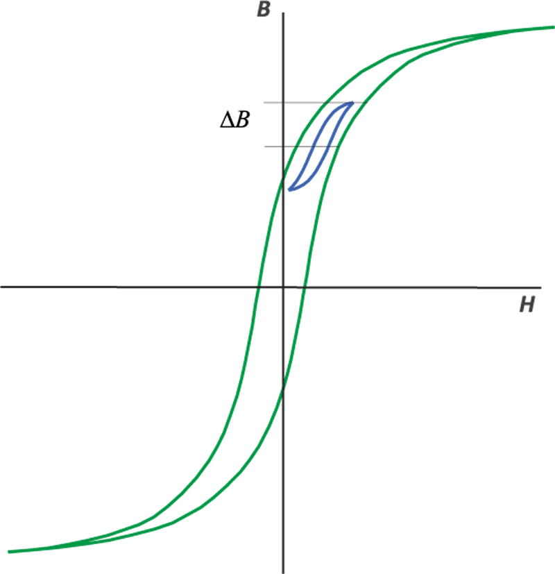
As frequencies climb beyond 50 kHz, core losses can start to become a significant source of loss in power supplies. Each time the core material is cycled around its B-H magnetization loop, there is energy loss. This is illustrated in Figure 1.

Click image to enlarge

Figure 1: B-H Loop for a High-Frequency Material

The green curve shows the core being driven all the way to saturation in each direction, positive and negative. Typically, this will not happen in a converter, and the flux excursion is stopped short of 0.3 T, well before the top of the curve flattens out.

The blue curve of Figure 1 shows a minor B-H loop with a DC bias. Notice that the loop is not as wide as the green curve, and the losses incurred each time around the loop are lower. This is a characteristic of magnetic cores. The harder they are driven, and the faster they are driven, the more the B-H curve opens up, and the higher the loss. The different magnetics in various different topologies will have great variations of excitations of their cores.

Measured core loss and the steinmetz equation

While the mechanisms for core loss have been the attention of much analysis and research in the past, there has not yet been a way to accurately predict the loss from just the chemical structure and physics of a material. Each time a new material is created for use by the power electronics industry, there must be extensive and careful characterization of the losses in the core material. This can only be done empirically.

The measurement of high-performance ferrite cores is a procedure that needs very accurate instrumentation in order to get good data. Calorimetry is still used as the most accurate technique. Extracting loss data from just electrical measurements does not have enough precision.

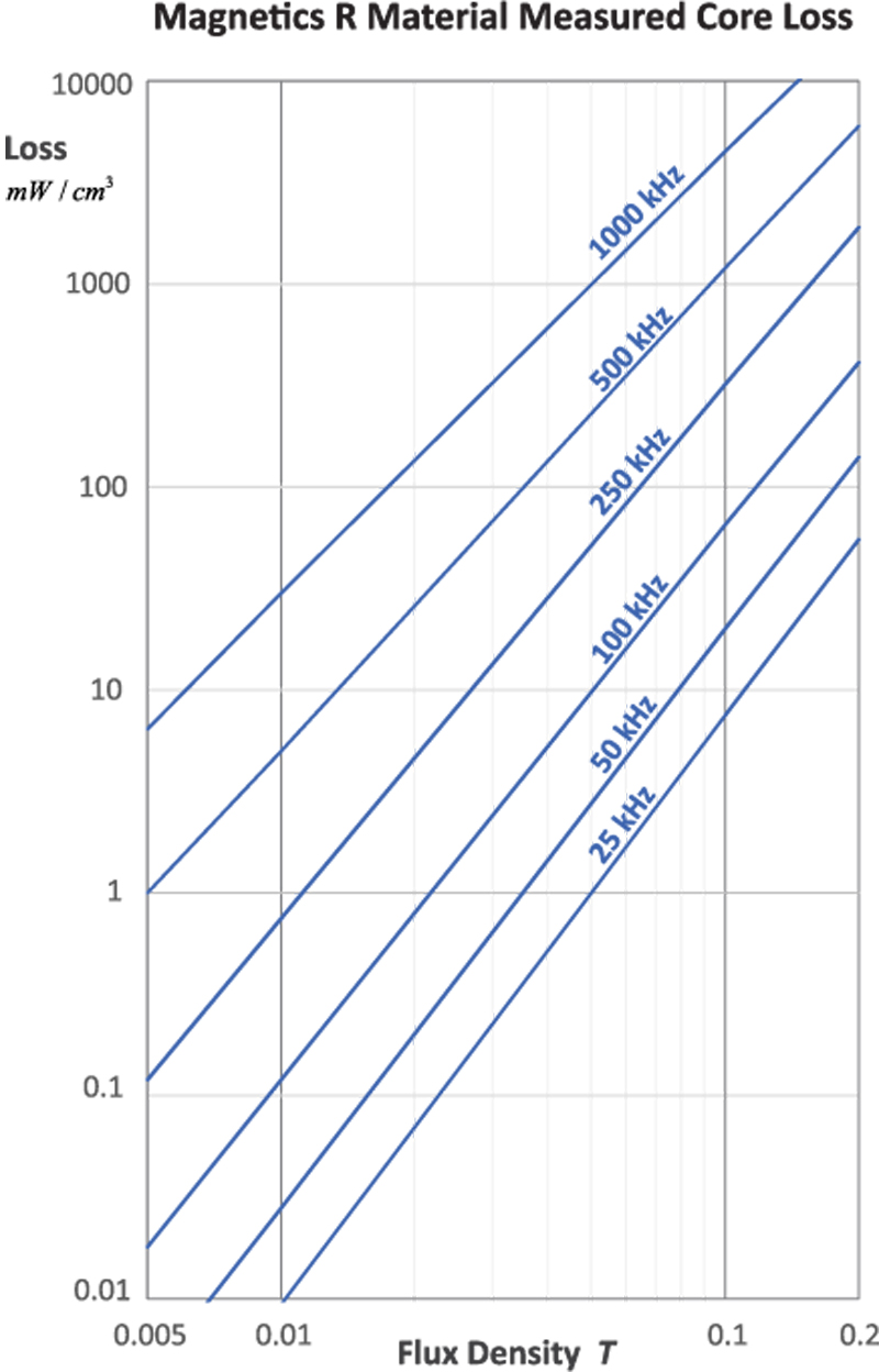
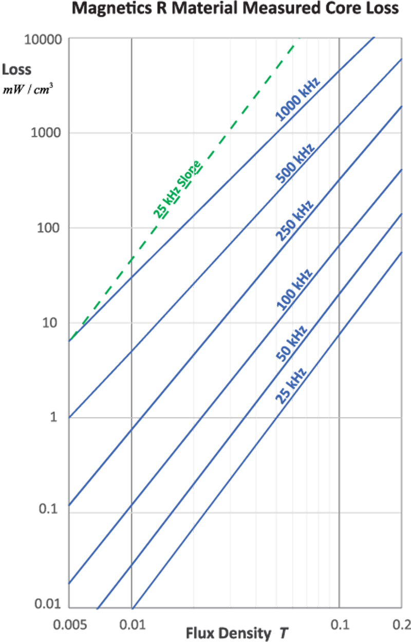
Figure 2 shows a family of loss measurements for Magnetics R material. To generate these curves, the core is driven sinusoidally to different flux levels over a range of frequencies from 25 kHz to 1000 kHz. Beyond 1 MHz, this material is not the best one to choose, although it can certainly still be used if the excitation levels are not too high.

Click image to enlarge

Figure 2: Typical Core Loss Measurements for Magnetics “R” Material

Empirical results for each core material give the most accurate data that can be obtained. Usually we rely on the core vendors to provide this data and it is not a process that you are likely to try and do yourself. However, curves are not particularly convenient to work with when trying to do computer-aided design.

In order to address this shortfall, we have the Steinmetz equation to predict what the core loss will be. Due to the nonlinear nature of core loss, this equation is somewhat unusual. The frequency exponent, c, in the equation is usually a number somewhere between 1 and 2.  (A value of 1 would result if the BH loop shape was fixed with frequency, but as mentioned before, it will grow larger at higher frequencies.)

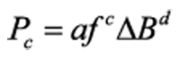
Equation 1: Steinmetz Equation for Core Loss

The ΔB exponent, d, in equation 1 would be equal to 2 if the only losses were due to classic core hysteresis. However nonlinear effects result in an exponent between 2 and 3.

Despite the popularity of the Steinmetz equation, it is of limited use in its normal fixed form. The frequency exponent is only fixed if the separation of frequency multiples is always the same. That is, the distance between the 25 kHz and 50 kHz curves of Figure 1 should be the same as the separation between the 500 kHz and 1000 kHz curves. This is clearly not the case. The separation is much larger at the higher frequencies.

The exponent for ΔB would be a constant value if the slopes of the loss curves were all the same, and at first glance, the curves of Figure 1 appear to be parallel to each other. However, this is something of an optical illusion. If you look at Figure 3, you will see the slope of the 25 kHz loss line, shown in green, compared to the 1000 kHz loss line. They are very different.

Click image to enlarge

Figure 3: Typical Core Loss Measurements for Magnetics “R” Material, Showing Slope Variations

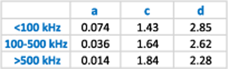
Since both of the exponents need to change with frequency, Magnetics Inc. provides a table of changing values, depending on the frequency range that is being used. This is repeated for you in Table 1. While this improves accuracy, it is cumbersome to use, and significant differences will be predicted in loss when the frequency changes from 99.9 kHz to 100.1 kHz.

Click image to enlarge

Table 1: Variable Coefficients Needed for Different Frequency Ranges

Core Loss and Ridley-Nace Modeling Formula

Another approach is possible to avoid using discretely-changing values for the exponents of the core loss equation. In 2006, we conducted research into better ways of modeling core losses with a continuous equation for all frequencies. This results in a fixed term for the frequency exponent, and frequency-dependent expressions for the constant and the ΔB exponent.

For the Magnetics R material, the resulting equation is shown below.

Equation 2: Ridley-Nace Formula for Core Loss

Figure 4 shows the result of using this equation. It isn’t perfect, but at the high-loss end of the curves, the fit is very good. Further refinement of the equation could be done, but this may not be the best immediate thing to do. Verification of the data would come first.

Click image to enlarge

Figure 4: Comparison of Measured Core Loss and Predicted Core Loss with Ridley-Nace Formula

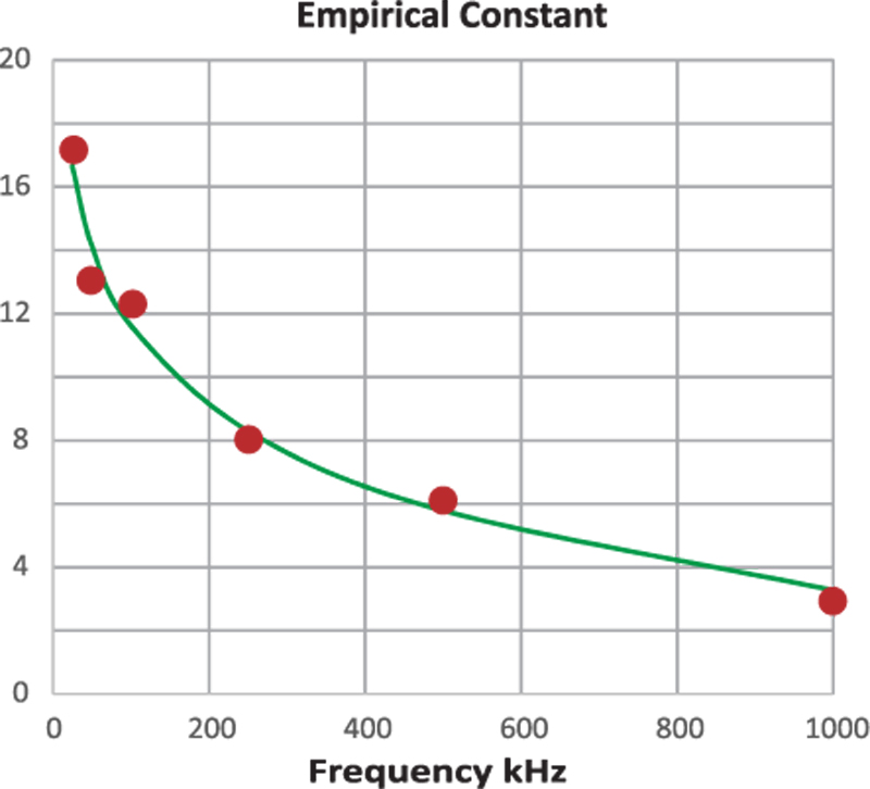
In Figure 5, you can see the curve-fitting procedure used to find the frequency-dependent constant of the new formula. This logarithmic function provides a good fit overall, but you can see that there are some data points that don’t seem to make complete sense, and they don’t complete a smooth curve. Before trying to improve the curve fitting, it would be important to verify the accuracy of the data. As mentioned before, this loss data is very difficult to measure accurately, and it is not surprising to see spurious results in the data points.

Click image to enlarge

Figure 5: Curve Fitting Used to Find the Constant for R Material in the Ridley-Nace Formula

Figure 6 shows the curve fitting used to find the flux exponent. Again, there are a couple of frequency points that seem to be outliers, and verification of the data would help improve the approximation to the measurements.

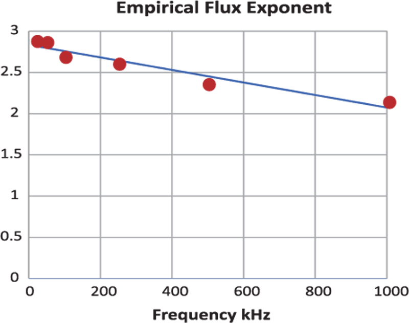
Click image to enlarge

Figure 6: Curve Fitting Used to Find Flux Exponent for R Material in Ridley-Nace Formula

The curve-fitting processes shown in Figures 5 and 6 can be done for any set of data for core loss. This has been done for many of the popular core materials, and the results have been incorporated into the program POWER 4-5-6.  

Looking forward

An improved form of the Steinmetz equation has been given for the R material ferrite. This new equation has a frequency-dependent constant, and a frequency-dependent exponent for the flux. Having a single expression for the core loss is tremendously useful for working with design programs and spreadsheets. As we will see in the next part of this article, it is invaluable for estimating the change in losses when non-sinusoidal waveforms with different duty cycles are encountered.

Ridley Engineering

References

[1]       Simulation and Design Software POWER 4-5-6 incorporating Ridley-Nace core-loss equation www.ridleyengineering.com/software/POWER_4-5-6_Manual.pdf

[2]       Power supply design articles www.ridleyengineering.com/design-center.html

[3]       Join our LinkedIn group titled “Power Supply Design Center”. Noncommercial site with over 5600 helpful members with lots of theoretical and practical experience. www.linkedin.com/groups?&gid=4860717

[4]       See our videos on power supply design at www.youtube.com/channel/UC4fShOOg9sg_SIaLAeVq19Q

[5]       Power supply design workshops including magnetics design www.ridleyengineering.com/workshops.html